“Where’s this special sauce?” CIA operative Bernadette in The Report asks psychologists James Mitchell and Bruce Jessen, after 60 days of waterboarding Muhammad Rahim yielded no results. “You have to make this work. It’s only legal if it works.”
Oracles, augurs, prophets, and pundits studied entrails, birds, and dreams looking for the special sauce, but the science of forecasting is young. A new article in the International Journal of Forecasting, which I wrote with colleagues Deniz Marti and Thomas Mazzuchi, claims to have found the special sauce—or at least some key ingredients—in the classical model for structured expert judgment. Torture isn’t among them.
Good expert forecasting does not correlate with citations, status, or blue ribbons. If you want to pick a good prophet, you look at her record. But her record of what? Tallying previous forecast errors isn’t as simple as it sounds. An error of three years in guessing the age of a Boeing-737 is not the same as an error of three years in guessing the age of your youngest daughter. Selecting forecasters based on previous errors requires converting errors to a common scale that accounts for the difference between aircraft years and daughter years.
Here’s the first key ingredient of the special sauce: the common scale is probability. How likely is an error of three aircraft years or three daughter years? That would be easy if we had a universal likelihood scale for all responses, but alas, we don’t. The next-best thing is the subjective probability of the expert forecaster herself. Suppose that for every forecast of a quasi-continuous unknown quantity, we tally how often the true value, revealed after the fact, falls within the expert’s 90 percent confidence bands.
Why would this help? Aren’t all experts pretty much equally able to assess how much they know? As it turns out, no. For some experts, saying they’re 90 percent certain that the true value falls in some interval confers a less than 10 percent chance of that predicted result actually happening. For other experts, you can take that 90 percent to the bank. Understanding an expert’s ability to gauge the likelihood of her own predictions might be good to know before we bet the farm on her advice.
Equipped with a common scale, we can reveal the second key ingredient of the special sauce: experts are not equal in their ability to quantify uncertainty. But how do we measure “the ability to quantify uncertainty,” and how we can use that information?
The third and perhaps most surprising sauce ingredient can help us: it’s better to combine expert uncertainties than to combine their point forecasts, and it’s better still to combine expert uncertainties based on their past performance.
An Example of These Principles in Action
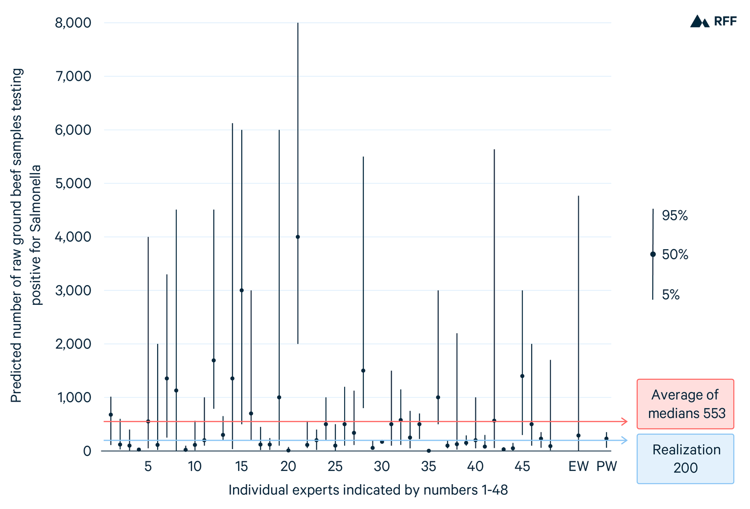
In a recent expert elicitation on foodborne illness pathways at the Centers for Disease Control and Prevention, one of the 14 calibration questions is the following: “Between January 1, 2016, and December 31, 2016, a total of 11,277 samples of raw ground beef from 1,193 establishments were tested for Salmonella spp. Of these samples, how many tested positive for Salmonella spp?” The medians and the 5th and 95th percentiles of the 48 participating experts are shown in Figure 1, as is the true value: 200 samples tested positive. Had we simply asked the experts for their best guesses, we would have gotten something like the average of the 48 median values, which is 553.
If we also ask for their 90 percent confidence bands, then we have the option of combining their distributions. If we weight the experts equally (equal weighting; EW) and take the median of this combined distribution, we get 286 predicted positive samples, with a 90 percent confidence band that ranges widely, between 1 and 4,769. We can also weight the experts based on their performance on all calibration variables (performance-based weighting; PW). The median of the PW combination is 230, with a 90 percent confidence band of 60–350.
Figure 1
Of course, this is just one example chosen to illustrate these features; we need more examples to draw accurate conclusions. Our article chronicles several applications of the classical model. Other highlighted examples of professional applications include nuclear safety with the European Union and the United States Nuclear Regulatory Commission; fine particulates with Harvard University and the government of Kuwait in 2004–2005; foodborne diseases for the World Health Organization in 2011–2013; ice sheet dynamics; and volcanic hazard, forecasts, and risk level assessments in different parts of the world. From 2006 to 2018, 49 commissioned applications have involved 530 experts, who are scored by assessing 580 calibration variables from their fields. The judgments of about 75 percent of these experts, considered as statistical hypotheses, would be rejected at the traditional 5 percent significance level.
What Have We Learned?
So, what have we learned? Is one expert as good as another? Are the measured performance differences just noise? This sounds like the beginning of a fruitless debate, but we can actually test the ideas with performance data.
Notice that performance-blind combination schemes, such as equal weighting, are unaffected if the assessments in an expert panel are randomly reallocated item-wise among the experts. Performance weighting depends on being able to identify high-performing experts. If we randomly reallocate the assessments, then any remaining performance differences will be due to noise.
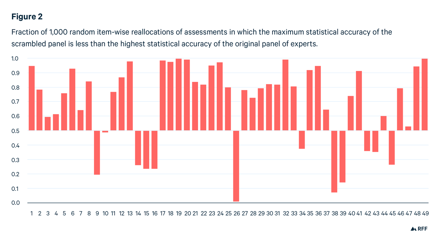
For each of the 49 studies, we repeat this random scrambling 1,000 times. How does the statistical accuracy of the best-performing expert in the original panel compare with the best performers in each of the 1,000 scrambled panels?
If there really is no difference between the real and scrambled best performers, then the real best performer could just as well be any of the 1,000 scrambled best performers: as such, he has a 50 percent chance of performing better than the median of the scrambled best performers, a 30 percent chance of outperforming 70 percent of the scrambled best performers, and so on. Among the 49 studies, we would expect the best performer to make better predictions than 70 percent of the other experts in 15 (i.e., 30 percent) of the studies. If we look at the data in Figure 2, we readily see that this is not the case. In 31 studies, the original best performer makes better predictions than 70 percent of the scrambled best performers. The probability of this result is 1.6E-6, if the differences are really due to random noise rather than to objectively better predictions by a subset of experts. Other performance metrics give a similar picture, and more powerful statistical tests bring the probability down to E-12 of seeing this result caused by noise. Thus, the performance differences among experts are real.
So, if experts quantify their uncertainty, we can combine their uncertainties and extract point predictions from the combinations, as in Figure 1. We can also quantify their performance as uncertainty assessors and use that information to form performance-weighted combinations of uncertainty. That led to a better point prediction in Figure 1. How does the method work out for all 580 assessments for which we know the true values?
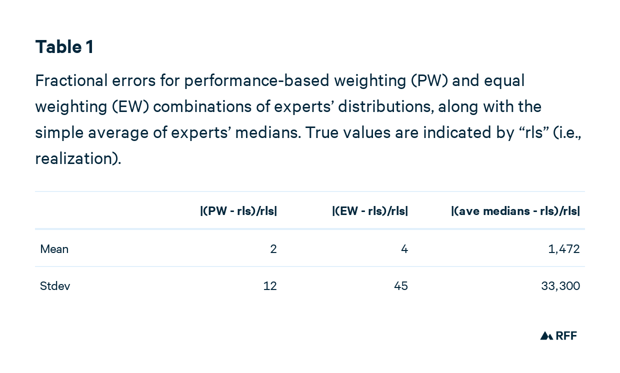
Once again, to compare predictions, we have to standardize for scale. One option is to use the fractional prediction error, |(prediction – realization)/realization)|, which works only if the realization (i.e., the true value) is nonzero. Table 1 compares the fractional prediction errors. Simply averaging experts’ medians is the clear loser, producing a prediction that’s way off base. Medians of equally weighted combinations of expert distributions is an improvement, but has a wider spread of outcomes. Figure 3 graphs these results.
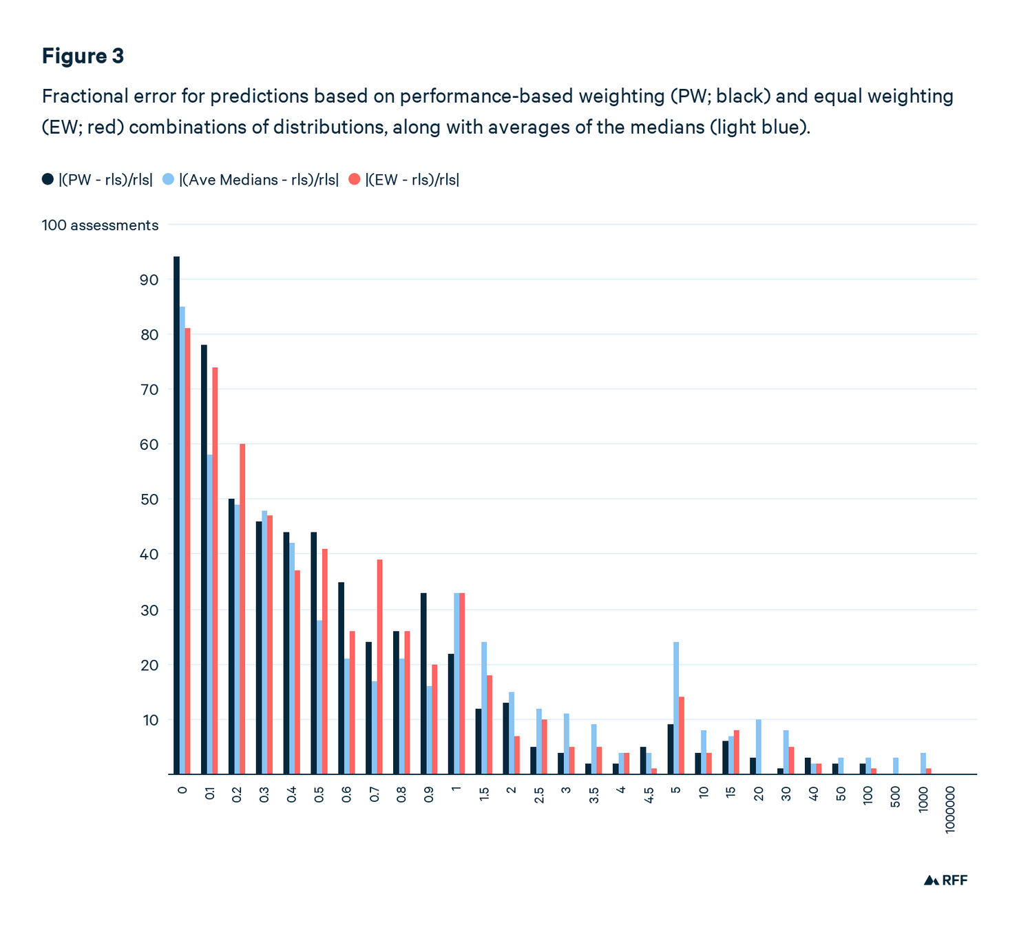
Of all the PW predictions, 48 have a fractional error greater than 2. In other words, if the true value were 200, the prediction would be greater than 600. For EW, there were 60 such predictions and for the simple average of medians, 112, or about 20 percent of all predictions.
All in all, we may have some special sauce, but we do not have a silver bullet.


